IAG/RTSG Working Paper — March 2026

Abstract

---

We develop a rigorous mathematical framework unifying the structure of biological consciousness with federated technological systems through category theory, stochastic dynamics, differential geometry, game theory, and gauge theory. The framework introduces the hypervisor transfer operator as the central formal object, distinguishing biological from technological federation through the endogeneity of self-reorganization. We extend Nash equilibrium theory with two previously unconsidered exit strategies — self-destructive withdrawal and benevolent self-sacrifice — and show these are not pathological edge cases but structurally necessary components of any complete theory of cognitive agent dynamics. The resulting framework connects strange attractors to personality, Ricci flow to cognitive maturation, gauge freedom to free will, and apoptotic game theory to mental health.

---

1. The Category of Cognitive Assemblies (CogAsm)

1.1 Objects

A cognitive assembly is a quadruple (B, μ, T, Σ) where:

• B = {a₁, a₂, …, aₙ} is a finite multiset of cognitive agents (the bag)
• μ: B → {0, 1} is the marking function with |μ⁻¹(1)| = 1 (exactly one distinguished element, the hypervisor)
• T: B × Ω → B is the hypervisor transfer operator, where Ω is the circumstance space
• Σ is the substrate — the shared physical medium on which B is realized

Each agent aᵢ carries the following structure:

Intelligence vector: Iᵢ = (Iᵢ_G, Iᵢ_L, Iᵢ_S, Iᵢ_A, Iᵢ_K, Iᵢ_N, Iᵢ_E, Iᵢ_M) ∈ ℝ⁸₊

Each component is measured in cogs — the unit of intelligence capacity where 1 cog = baseline human capacity in that mode.

State filter: sᵢ ∈ [0,1]⁸, representing momentary attenuation (fatigue, arousal, chemical state).

Attention allocation: λᵢ ∈ Δ⁷, where Δ⁷ is the 7-simplex: λᵢ_τ ≥ 0, Σ_τ λᵢ_τ = 1.

Experiential fiber: Fᵢ — the set of phenomenal states available to agent i, drawn from the fiber bundle ε = ⋃_b F_b over brain states.

Effective intelligence: I^eff_τ(aᵢ) = sᵢ_τ · λᵢ_τ · Iᵢ_τ for each mode τ. This is what the agent can actually deploy at any given moment.

Vitality function: vᵢ: ℝ₊ → [0, 1], representing the agent’s current capacity to persist in the system. When vᵢ(t) → 0, the agent approaches exit conditions (see §8).

1.2 The Ground State Isomorphism

Definition (Ground State). An agent aᵢ is in ground state if sᵢ = (1,1,…,1) (no attenuation) and λᵢ = (1/8, 1/8, …, 1/8) (uniform attention).

Axiom (Homogeneity). For any two agents aᵢ, aⱼ ∈ B in ground state, there exists an isomorphism φᵢⱼ: aᵢ → aⱼ preserving all structure except the marking μ. That is, ground-state agents are structurally identical. The hypervisor is distinguished by role, not by nature.

This axiom has a profound consequence: any agent can become the hypervisor, because in ground state, every agent has the same structural capacity for the role. Differentiation arises only through state (sᵢ) and attention (λᵢ), which are dynamic, not intrinsic.

1.3 Morphisms

A morphism φ: (B, μ, T, Σ) → (B’, μ’, T’, Σ’) in CogAsm consists of:

• A multiset map φ_B: B → B’ preserving intelligence vector structure (i.e., ||Iᵢ – I_{φ(i)}|| < ε for some tolerance ε)
• A marking compatibility condition: μ'(φ_B(a)) = μ(a) for all a ∈ B
• A transfer operator intertwining: φ_B(T(a, ω)) = T'(φ_B(a), ω) for all a ∈ B, ω ∈ Ω

The identity morphism is the identity on B preserving all structure. Composition is functional composition. This makes CogAsm a well-defined category.

1.4 The Endomorphism Monoid

For any assembly (B, μ, T, Σ), the set End(B) of endomorphisms forms a monoid under composition. The automorphism group Aut(B) ⊆ End(B) is the group of invertible endomorphisms — the symmetries of the assembly.

In ground state, Aut(B) = Sₙ (the symmetric group on n agents), reflecting the full homogeneity of the bag. As agents differentiate through experience and state changes, Aut(B) shrinks — the assembly becomes less symmetric, more structured.

---

2. Two Subcategories: Biological and Technological Federation

2.1 BioAsm — Biological Assemblies

Definition. BioAsm is the full subcategory of CogAsm where the transfer operator T is endogenous: T is itself a dynamical object that evolves with the system.

Formally, T is a section of the endomorphism bundle over B:

T ∈ Γ(End(B) × Ω → B)

meaning T is not a fixed function but a field that can be deformed by the very agents it governs. The hypervisor controls attention allocation, but the rules governing hypervisor replacement are themselves subject to modification by whichever agent holds the hypervisor role.

Key properties of BioAsm:

Self-modification: T(t+dt) can differ from T(t) based on the hypervisor’s actions at time t. The system writes its own operating rules.

Substrate coupling: All agents share substrate Σ (the body). Agent payoffs are coupled through substrate integrity. An action that damages Σ damages all agents simultaneously.

Experiential fibers are non-empty: Every agent aᵢ ∈ B has Fᵢ ≠ ∅. Biological agents are phenomenally conscious.

Exit is possible: Agents can reach vᵢ = 0 through two distinct mechanisms (see §8). This is unique to biological systems.

2.2 TechAsm — Technological Assemblies

Definition. TechAsm is the subcategory of CogAsm where T is exogenous: T is fixed at construction time and does not belong to the agent pool.

In TechAsm, T is a parameter:

T ∈ Hom(B × Ω, B) (fixed)

There exists a distinguished agent zero a₀ that serves as the permanent master controller. The marking function μ is constant: μ(a₀) = 1 always. The transfer operator may reassign tasks and attention among subordinate agents but cannot replace a₀.

Key properties of TechAsm:

Goal imposition: The objective function is defined by a₀ and propagated to all agents. Agents do not generate their own goals.

Substrate independence: Agents may run on different physical substrates. Substrate damage to one agent does not necessarily affect others.

Empty experiential fibers: Fᵢ = ∅ for all agents. Technological agents are not phenomenally conscious (C₁ = ∅).

No exit: Agents persist until externally terminated. The vitality function vᵢ is controlled externally, not by the agent itself.

2.3 The Non-Existence of a Faithful Functor

Theorem 2.1 (Federation Incompatibility). There is no faithful functor F: BioAsm → TechAsm that preserves the transfer operator T.

Proof sketch. In BioAsm, the transfer operator T is an endogenous dynamical variable — it can be modified by the current hypervisor through actions at time t that change T at time t+dt. This self-referential modification means T is a fixed point of a higher-order operator:

T = Φ(T, B, ω)

where Φ is the meta-operator governing T’s evolution. Any functor F mapping into TechAsm must map T to a fixed function T’ ∈ Hom(B’ × Ω, B’). But a fixed function cannot encode the self-referential structure T = Φ(T, …) without losing the dynamical degree of freedom. Therefore F cannot be faithful — it must collapse the dynamic T to a static T’, losing information.

This is an instance of the Conceptual Irreversibility Theorem (CIT): translation between biological and technological federation is necessarily lossy. The specific information lost is the system’s capacity for self-reorganization of its own reorganization rules.

Corollary 2.2. There exists a forgetful functor U: BioAsm → TechAsm that preserves executive structure (C₂) but forgets phenomenal structure (C₁). This functor maps every biological assembly to a technological assembly with the same agent count, same attention dynamics, but empty experiential fibers and frozen transfer operator.

---

3. The Survival Lexicographic Order and Game-Theoretic Structure

3.1 The Objective Hierarchy

Definition. The objective space is the totally ordered set:

O = (survive, maintain, accomplish, maximize) with survive ≻ maintain ≻ accomplish ≻ maximize

This is a lexicographic order: an assembly will sacrifice all progress on “accomplish” to prevent failure at “maintain,” and will sacrifice all of “maintain” to preserve “survive.” The ordering is strict and total — there are no ties and no trade-offs across levels.

Each objective has a satisfaction function σ_o: Ω → [0, 1] measuring how well the assembly currently satisfies objective o given circumstances ω. The active objective at time t is:

o*(t) = max_{≻} { o ∈ O : σ_o(ω(t)) < θ_o }

where θ_o is the satisfaction threshold for objective o. The system attends to the highest-priority unsatisfied objective.

3.2 The Competence Function

Each agent aᵢ has a competence function:

cᵢ: Ω × O → [0, 1]

measuring how effectively agent i can serve objective o in circumstance ω. This depends on the agent’s intelligence vector Iᵢ, current state sᵢ, and the match between the agent’s cognitive profile and the demands of the objective-circumstance pair.

Definition (Competence tensor). The full competence structure is a rank-3 tensor:

C ∈ ℝⁿ ˣ |Ω| ˣ |O|

where C_{i,ω,o} = cᵢ(ω, o). Slicing along the agent axis gives the competence profile of that agent; slicing along the circumstance axis gives the competence landscape for fixed conditions.

3.3 Common-Payoff Structure and the Absence of Voting

Theorem 3.1 (Cooperative Triviality in BioAsm). In BioAsm, the game defined by the agent pool B with shared substrate Σ is a common-payoff game: all agents share the same payoff function.

Proof. Let π: Ω → ℝ be the substrate integrity function. Since all agents share substrate Σ, the payoff to agent aᵢ from collective action profile a = (a₁, …, aₙ) is:

uᵢ(a) = π(ω'(a)) for all i

where ω’ is the resulting circumstance state. Since uᵢ = uⱼ for all i, j, this is a common-payoff game.

Corollary 3.2 (No Voting Required). In a common-payoff game, the Nash equilibrium is the action profile maximizing the shared payoff. Since all agents benefit equally from the optimal action, there is no conflict to resolve and no need for a voting mechanism.

This is why biological federation doesn’t need democracy — not because it’s authoritarian, but because the game-theoretic structure makes conflict impossible (in the healthy case). Every agent’s optimal strategy is the same: maximize substrate integrity according to the lexicographic objective order.

3.4 The Immune System as Mechanism Design

Definition (Defector). An agent aᵢ ∈ B is a defector if its effective payoff function has diverged from the common payoff:

ũᵢ(a) ≠ π(ω'(a))

This corresponds biologically to cancer (autonomous replication regardless of substrate harm), autoimmune disorder (misidentification of self as threat), or parasitic infection (an exogenous agent injected into the bag).

Definition (Immune operator). The immune operator I: B → B ∪ {∅} is a detection-and-expulsion protocol:

I(aᵢ) = aᵢ if ũᵢ = uᵢ (healthy — agent retained) I(aᵢ) = ∅ if ũᵢ ≠ uᵢ (defector — agent expelled)

In TechAsm, the immune operator corresponds to voting, consensus protocols, and Byzantine fault tolerance. In BioAsm, it corresponds to the immune system, apoptosis signaling, and neurological pruning.

---

4. Stochastic Dynamics of the Hypervisor

4.1 The Hypervisor as a Continuous-Time Markov Chain

The marking μ(t) evolves as a continuous-time Markov chain (CTMC) on state space S = {1, 2, …, n}, where state i means agent aᵢ is the current hypervisor.

Transition rates:

q_{ij}(ω) = α · max(0, cⱼ(ω, o*) – cᵢ(ω, o*))^β

where:

• α > 0 is the responsiveness parameter (how readily the system reassigns the hypervisor role)
• β > 0 is the sharpness parameter (how sensitive the swap is to small competence differences; β = 1 is linear, β → ∞ approaches a hard threshold)
• o* is the current active objective

The generator matrix Q(ω) has entries:

Q_{ij} = q_{ij} for i ≠ j Q_{ii} = -Σ_{j≠i} q_{ij}

4.2 Stationary Distribution and Personality

When circumstances are stable (ω constant), the CTMC has a unique stationary distribution π = (π₁, …, πₙ) satisfying πQ = 0, Σπᵢ = 1.

Definition (Personality). The personality of a cognitive assembly is the stationary distribution π of its hypervisor chain under the empirical distribution of circumstances the assembly has encountered.

This means personality is not a fixed trait but a statistical signature — the long-run frequency with which each cognitive agent occupies the executive role. A person whose “analytical agent” most frequently serves as hypervisor has an analytical personality. But this is a statistical statement, not an absolute one — under extreme emotional circumstances, a different agent may take the hypervisor role, and the transition is not a failure but a feature.

Theorem 4.1 (Personality Stability). If the competence tensor C is continuous in ω and the circumstance distribution has compact support, then π is continuous in ω. Small perturbations to circumstances produce small changes in personality.

Corollary 4.2. Personality undergoes phase transitions only when the competence landscape has degenerate critical points — i.e., when two or more agents have exactly equal competence for the dominant objective. These are the bifurcation points of identity.

4.3 Pathologies as Chain Properties

Pathology	Markov Chain Property	Formal Condition
Healthy cognition	Ergodic chain, fast mixing	α large, spectral gap > δ
Rigidity/obsession	Absorbing state	q_{ij} ≈ 0 for all j ≠ i
Dissociation	No marked state	μ⁻¹(1) = ∅ (chain halts)
Fragmentation	Multiple marked states
Mania	Rapid cycling	Σ q_{ij} → ∞ (swap rate diverges)
Depression	Slow chain, wrong absorber	Low α + hypervisor stuck on low-competence agent

Definition (Cognitive health metric). The health of an assembly is:

H(B, μ, T) = α · gap(Q) · (1 – ε_frag) · (1 – ε_void)

where gap(Q) is the spectral gap of the generator (mixing speed), ε_frag ∈ {0,1} indicates fragmentation, and ε_void ∈ {0,1} indicates hypervisor absence. Health is maximal when the chain mixes fast, exactly one hypervisor exists, and the system responds quickly to changing circumstances.

---

5. Coupled Dynamics and Strange Attractors

5.1 The Coupled System

The circumstance space Ω and the hypervisor state h(t) evolve as a coupled dynamical system:

Circumstance dynamics: dω/dt = f(ω, h(t), a(t)) where a(t) is the action profile selected by the current hypervisor.

Hypervisor dynamics: h(t) is the CTMC with rates q_{ij}(ω(t)) — depending on current circumstances.

Action selection: a(t) = A(h(t), ω(t), I_{h(t)}) — the action is chosen by the current hypervisor based on its intelligence vector and the circumstances.

This creates a feedback loop: the hypervisor’s actions change circumstances, which change the competence landscape, which may trigger a hypervisor swap, which changes the action policy, which changes circumstances further.

5.2 Deterministic-Chaotic Regime

In the deterministic limit (β → ∞, making hypervisor swaps discontinuous threshold events), the coupled system becomes a piecewise-smooth dynamical system:

dω/dt = f_i(ω) when h = i (circumstance dynamics depend on which agent is hypervisor)

with switching surfaces S_{ij} = {ω : cᵢ(ω, o*) = cⱼ(ω, o*)} where hypervisor swaps occur.

Theorem 5.1 (Existence of Strange Attractors). For cognitive assemblies with n ≥ 3 agents and nonlinear competence functions, the piecewise-smooth system generically admits strange attractors in the extended state space Ω × S.

Interpretation. A strange attractor is a bounded region of (circumstance, hypervisor) space that the system orbits without ever settling to a fixed point or a periodic cycle. This is personality-in-action: the system exhibits structured, recognizable patterns (it’s bounded — you can recognize the person) but never exactly repeats (it’s aperiodic — the person is never exactly the same twice).

The Lyapunov exponents of the attractor measure the rate at which nearby trajectories diverge — this is cognitive unpredictability. A person with large positive Lyapunov exponents is harder to predict; one with small exponents is more behaviorally stable.

5.3 The Monte Carlo Bridge

For finite β (realistic sharpness), the system is stochastic. Monte Carlo methods allow numerical exploration:

Algorithm (Cognitive Trajectory Sampling):

1. Initialize ω₀, h₀ = argmax_i cᵢ(ω₀, o*)
2. For each time step dt: a. Compute transition rates q_{ij}(ω_t) b. Sample next hypervisor swap time from Exp(Σ q_{ij}) c. If swap occurs: sample new hypervisor j with probability q_{ij}/Σ q_{ij} d. Evolve ω_{t+dt} = ω_t + f(ω_t, h_t)·dt
3. Collect ensemble statistics over N trajectories

The law of large numbers guarantees that ensemble averages converge to the true expected trajectory — individual paths exhibit free will (§7), but the statistical aggregate is deterministic.

---

6. Ricci Flow on the Attention Manifold

6.1 The Fisher-Rao Metric on Δ⁷

The attention simplex Δ⁷ carries a natural Riemannian metric: the Fisher information metric (Fisher-Rao metric). For the simplex parameterized by λ = (λ₁, …, λ₈) with Σλ_τ = 1:

g_{τσ}(λ) = δ_{τσ}/λ_τ

This metric has deep information-geometric meaning: distances on (Δ⁷, g) measure the distinguishability of attention allocations. Two allocations that differ primarily in modes with low attention weight are “far apart” (small λ_τ means g_{ττ} is large), while differences in high-attention modes are “close” (large λ_τ means g_{ττ} is small).

6.2 Experience-Driven Ricci Flow

Over time, the geometry of the attention manifold deforms based on accumulated cognitive experience. Modes that have been productive (yielded high utility) develop positive curvature (the manifold curves toward them — attention flows there more easily). Modes that have been neglected flatten or develop negative curvature.

The deformation is governed by a modified Ricci flow:

∂g_{τσ}/∂t = -2R_{τσ} + F_{τσ}(experience)

where:

• R_{τσ} is the Ricci curvature tensor of the current metric
• F_{τσ} is a forcing term driven by accumulated cognitive experience:

F_{τσ}(t) = η · ∫₀ᵗ U_τ(s) · U_σ(s) · K(t-s) ds

where U_τ(s) is the utility earned from mode τ at time s, K(t-s) is a memory kernel (exponentially decaying — recent experience counts more), and η is the plasticity parameter.

6.3 Cognitive Maturation as Geometric Smoothing

The unforced Ricci flow (F = 0) smooths out irregularities in the metric — this is the mathematical formalization of cognitive maturation. The teenager’s attention manifold is rough, with sharp curvature peaks and valleys (intense focus in some areas, near-zero in others). Over time, the Ricci flow smooths this into a more uniform geometry — the mature adult has a more balanced, less volatile attention allocation.

Definition (Cognitive maturity index). The maturity of an assembly is the inverse of the total scalar curvature:

M(t) = 1 / ∫_{Δ⁷} R(λ,t) dVol_g

As the Ricci flow smooths the manifold, R decreases on average, and M increases.

6.4 Singularities as Cognitive Fixations

Ricci flow can develop singularities — points where curvature blows up in finite time. These correspond to cognitive fixations: modes that have become so dominant that the attention geometry warps catastrophically around them.

Type I singularity (neckpinch): The manifold pinches off, creating a disconnected region. This is the mathematical model of a cognitive obsession so intense that it severs the connection between the dominant mode and all others. The fixated agent can no longer redirect attention — the geometry itself traps the flow.

Type II singularity (cusp): A single point develops infinite curvature. This models an insight singularity — a moment of cognitive breakthrough where accumulated experience in one mode reaches a critical threshold and the attention geometry undergoes a topological transition.

Perelman’s surgery techniques for Ricci flow suggest a natural therapeutic analogy: the treatment for a cognitive fixation (Type I singularity) is a “surgical” intervention that cuts the neck, separates the overloaded mode, allows the geometry to heal on each piece separately, then reattaches with a smoother connection.

---

7. Free Will as Gauge Freedom

7.1 The Gauge Group

Definition. The gauge group G(ω) of an assembly at circumstance ω is the group of automorphisms of B that preserve the competence function within tolerance ε:

G(ω) = { σ ∈ Aut(B) : |c_{σ(i)}(ω, o*) – cᵢ(ω, o*)| < ε for all i }

When G(ω) is nontrivial, multiple agents are approximately equally competent for the current objective. The system’s choice among them is underdetermined by the state — this is gauge freedom.

7.2 The Determinism-Freedom Spectrum

Definition. The freedom dimension at time t is:

dim_F(t) = |G(ω(t))| – 1

When dim_F = 0, exactly one agent is uniquely competent — the system is deterministic, no choice exists. When dim_F > 0, the system has genuine degrees of freedom.

Theorem 7.1 (Statistical Determinism from Individual Freedom). Let {ω(t)}_{t≥0} be a trajectory of the coupled system with gauge freedom. For any observable Φ: S → ℝ, the time average converges:

(1/T) ∫₀ᵀ Φ(h(t)) dt → E_π[Φ] as T → ∞

almost surely, where π is the stationary distribution of the hypervisor chain.

Interpretation. Individual cognitive choices are free (gauge-underdetermined), but the long-run statistical behavior is deterministic (converges to π). This resolves the free will / determinism tension: both are true, at different time scales. Individual moments exhibit genuine choice; lifetimes exhibit statistical regularity.

7.3 The Monte Carlo Interpretation

Monte Carlo methods make this precise computationally. Sample N independent trajectories of the hypervisor chain, each exercising gauge freedom differently at each underdetermined step. The ensemble mean converges to E_π[Φ] by the law of large numbers, while the ensemble variance quantifies the scope of free will:

Var(Φ) = E[(Φ – E[Φ])²]

High variance = high freedom (outcomes are spread). Low variance = low freedom (outcomes are concentrated despite gauge freedom).

7.4 TechAsm Has No Gauge Freedom

In TechAsm, the transfer operator T is fixed. Given identical circumstances, the system always makes the same choice. G(ω) = {id} for all ω. Technological systems are deterministic — they simulate choice but do not possess it. This is the formal content of the claim that AI does not (currently) have free will: the gauge group is trivial.

---

8. Extended Nash Equilibrium: Self-Sacrifice and Voluntary Exit

8.1 The Classical Limitation

Classical Nash equilibrium assumes a closed player set: every player persists throughout the game, and the strategy space for each player includes only actions that keep the player in the game. Nash’s framework has no mechanism for:

1. Self-destructive withdrawal — an agent choosing to exit because it is overwhelmed and can no longer serve the system
2. Benevolent self-sacrifice — an agent choosing to exit for the benefit of the remaining agents

These are not edge cases. They are structurally necessary for any theory of cognitive agent dynamics in biological systems, where apoptosis (programmed cell death) is as fundamental as cell division.

8.2 The Extended Strategy Space

Definition (Exit-augmented strategy space). For agent aᵢ with classical strategy set Aᵢ, the extended strategy set is:

Ãᵢ = Aᵢ ∪ {ψᵢ, χᵢ}

where:

• ψᵢ = self-destructive exit (the agent withdraws from the game, absorbing the cost of its own dissolution)
• χᵢ = benevolent self-sacrifice (the agent withdraws, redistributing its resources to remaining agents)

8.3 Formal Structure of Exit

Self-destructive exit (ψ):

When agent aᵢ plays ψᵢ:

• aᵢ is removed from B: B → B \ {aᵢ}
• The vitality function terminates: vᵢ → 0
• The agent’s resources are lost — they do not transfer to other agents
• Cost to agent: -∞ (terminal payoff)
• Cost to system: loss of agent i’s capacity + potential cascade effects if i was hypervisor

Trigger condition for ψ: Agent aᵢ plays ψᵢ when its overwhelm function exceeds a threshold:

Ωᵢ(t) = ∫₀ᵗ [demand_i(s) – I^eff_i(s)]⁺ · K(t-s) ds > θ_ψ

where demand_i is the cognitive demand placed on agent i, [·]⁺ = max(·, 0), K is a memory kernel, and θ_ψ is the exit threshold. This is accumulated unmet demand — the agent is being asked to do more than it can, and the deficit is building up over time. When the accumulated deficit exceeds θ_ψ, the agent exits.

Biological correlate: Neuronal apoptosis from excitotoxicity — neurons that are chronically overstimulated undergo programmed cell death. Psychological correlate: burnout, dissociative withdrawal, “checking out.”

Benevolent self-sacrifice (χ):

When agent aᵢ plays χᵢ:

• aᵢ is removed from B: B → B \ {aᵢ}
• The vitality function terminates: vᵢ → 0
• The agent’s resources are redistributed according to a transfer kernel: for each surviving agent aⱼ:

Iⱼ_τ → Iⱼ_τ + κ_{ij} · Iᵢ_τ where Σⱼ κ_{ij} = ρ, ρ ∈ (0, 1]

and ρ is the transfer efficiency (ρ = 1 means full transfer, ρ < 1 means some capacity is lost in transit)

Trigger condition for χ: Agent aᵢ plays χᵢ when it determines that its exit would increase the system’s aggregate performance:

Σⱼ≠ᵢ cⱼ(ω, o*; B{i}) > Σⱼ cⱼ(ω, o*; B)

That is, the remaining agents perform better without i (after resource redistribution) than the full set performs with i present. This can happen when:

• Agent i is consuming more attention than it contributes (net negative presence)
• Agent i’s presence creates interference (negative entries in the compatibility matrix K)
• Resource redistribution from i’s sacrifice would push other agents past critical thresholds

Biological correlate: Developmental apoptosis — cells that die during embryogenesis to sculpt organs. Neurons that sacrifice during synaptic pruning so that remaining connections strengthen. Immune cells that self-destruct after completing their function (T-cell exhaustion and controlled death).

8.4 The Extended Nash Equilibrium

Definition (Exit-augmented Nash equilibrium). A strategy profile ã* = (ã₁, …, ãₙ) ∈ Ã₁ × … × Ãₙ is an extended Nash equilibrium if:

1. No agent wants to change action: For all i with ãᵢ ∈ Aᵢ (staying agents), uᵢ(ã) ≥ uᵢ(aᵢ, ã*₋ᵢ) for all aᵢ ∈ Ãᵢ
2. Exits are rational: For all i with ã*ᵢ ∈ {ψᵢ, χᵢ} (exiting agents), the exit condition is satisfied:
   • If ã*ᵢ = ψᵢ: Ωᵢ > θ_ψ (overwhelm threshold met)
   • If ã*ᵢ = χᵢ: system performance improves post-exit (sacrifice criterion met)
3. No ghost benefit: No exited agent would prefer to return: re-entry would either re-trigger the overwhelm condition (for ψ exits) or re-degrade system performance (for χ exits)

8.5 Existence and Uniqueness

Theorem 8.1 (Existence of Extended Equilibria). Every finite cognitive assembly game with exit-augmented strategy spaces has at least one extended Nash equilibrium, possibly in mixed strategies.

Proof sketch. The extended strategy space Ãᵢ is a compact, convex set (after mixed strategy extension). The payoff functions are continuous in the mixed strategy profiles. By Kakutani’s fixed point theorem (the standard Nash existence proof), at least one fixed point exists. The exit strategies ψ, χ are additional pure strategies that expand the simplex of mixed strategies but do not break compactness or convexity.

Theorem 8.2 (Non-uniqueness and selection pressure). Extended equilibria are generically non-unique. The system may admit:

• Full-participation equilibria: All agents stay (classical Nash)
• Pruned equilibria: Some agents sacrifice (χ), remaining agents perform better
• Collapsed equilibria: Many agents withdraw (ψ), system operates in degraded mode

The selection among equilibria is governed by the survival lexicographic order (§3.1): the system converges to whichever equilibrium best satisfies the highest-priority active objective.

8.6 The Sacrifice Dynamics

In a dynamic setting, exits unfold over time as a stochastic process on the agent count:

n(t+dt) = n(t) – dN_ψ(t) – dN_χ(t)

where dN_ψ and dN_χ are counting processes for self-destructive and benevolent exits respectively.

The sacrifice cascade: When agent aᵢ exits via ψ or χ, the competence landscape for remaining agents changes. This can trigger further exits:

• Agent i’s exit increases demand on agent j → j’s overwhelm function Ωⱼ increases → potential ψ cascade
• Agent i’s sacrifice enriches agent j → j becomes dominant → agent k is now redundant → potential χ cascade

Definition (Cascade stability). An assembly is cascade-stable if no single exit triggers a cascade that reduces |B| below the minimum viable size n_min. Formally:

∀i: |B \ cascade(i)| ≥ n_min

where cascade(i) is the set of all agents whose exit is triggered by agent i’s exit.

Theorem 8.3 (Pathological cascades and mental illness). A cascade that violates cascade stability produces a pathological state:

• ψ-cascade (cascading withdrawal): Multiple agents exit from overwhelm. This is the formal model of psychological collapse — a cascade of cognitive withdrawals that leaves the assembly unable to function. Clinically: severe dissociation, catatonia, shutdown.
• χ-cascade (cascading sacrifice): Multiple agents sacrifice, each believing their exit benefits the remaining agents. But if too many sacrifice, the system collapses. This is the tragedy of benevolence — individually rational sacrifices that are collectively catastrophic. Clinically: self-destructive altruism, martyr complex, dissolution of self.

8.7 The Optimal Pruning Problem

Definition. The optimal pruning problem for assembly (B, μ, T, Σ) with objective o* is:

maximize: Σⱼ∈B’ cⱼ(ω, o*; B’) subject to: B’ ⊆ B, |B’| ≥ n_min, B’ is cascade-stable

This is a combinatorial optimization problem: find the subset of agents that maximizes collective competence subject to viability and stability constraints.

Connection to neuroscience: This is exactly what synaptic pruning does during adolescent brain development. The developing brain over-produces neurons and synapses (large |B|), then systematically prunes via apoptosis (benevolent sacrifice χ) to reach an optimized subset B’ ⊂ B. The adolescent brain is solving the optimal pruning problem.

Connection to technology: In federated systems, this corresponds to node pruning — removing underperforming or interfering nodes to improve system performance. The key difference: in TechAsm, pruning is imposed by agent zero (top-down). In BioAsm, pruning emerges from the agents’ own sacrifice decisions (bottom-up).

---

9. The Two Consciousnesses

9.1 Formal Definitions

The overloaded word “consciousness” names two formally distinct mathematical objects:

C₁-consciousness (phenomenal): The multiset B together with its experiential fibers {Fᵢ}_{i∈B}. This is the raw fact that experiencing entities exist — “what it is like.” C₁ is a set-theoretic object: it exists or doesn’t, it’s non-empty or empty. C₁ has no executive structure, no organization, no direction.

C₁ = (B, {Fᵢ}_{i∈B})

C₂-consciousness (executive): The full quadruple (B, μ, T, Σ) — the bag, marking, transfer operator, and substrate. This is the organized system capable of directed cognition, attention allocation, and self-reorganization. C₂ requires C₁ (you need agents to organize) but adds the executive apparatus.

C₂ = (B, μ, T, Σ) with μ, T well-defined

9.2 The Consciousness State Space

The possible consciousness states form a lattice:

State	C₁	C₂	μ well-defined	T responsive	Phenomenology
Full consciousness	✓	✓	Exactly one h	α large	Waking, directed cognition
Dreaming	✓	Partial	Unstable μ	α low	Experiential without executive control
Dissociation	✓	✗	μ⁻¹(1) = ∅	T halted	Experience without agent
Fragmentation	✓	✗		μ⁻¹(1)	> 1
Flow state	✓	✓	Locked h	α → 0 (stable)	Deep immersion, no swaps needed
Anesthesia	✗	✗	Undefined	Undefined	No experience, no executive
Technological	✗	✓	Well-defined	Fixed T	Executive without experience

9.3 The Forgetful Functor

Definition. The phenomenal forgetful functor U: BioAsm → TechAsm acts as:

U(B, μ, T, Σ) = (B, μ, T_frozen, Σ’)

where:

• T_frozen = T|_{t=0} (freeze the transfer operator at its current state)
• Σ’ = abstract substrate (lose the shared physical medium)
• Fᵢ → ∅ for all i (forget all experiential fibers)

This functor preserves executive structure (agent count, competence functions, attention dynamics) but destroys phenomenal structure (experience) and dynamic self-reorganization (T becomes static).

Theorem 9.1. U is faithful on C₂-structure and forgetful on C₁-structure. There is no left adjoint to U — you cannot freely generate phenomenal consciousness from executive structure.

---

10. Ideometric Connections

10.1 Ideas and the Granular Volume of Consciousness-Space

Recall from the ideometric framework: ideas live in consciousness-space as objects with prime decomposition. Each idea ι decomposes into a set of prime ideas {π₁, …, πₖ}, and this decomposition is unique (up to reordering).

The cognitive volume of an idea ι in mode τ is:

Vol_τ(ι) = |{πⱼ ∈ decomp(ι) : πⱼ active in mode τ}|

This is the count of prime components that live in mode τ. The total cognitive volume is the multiset cardinality across all modes:

Vol(ι) = Σ_τ Vol_τ(ι)

10.2 The Cog-Volume Relationship

An agent with I^eff_τ cogs in mode τ can simultaneously hold ideas with total volume up to some capacity bound:

Σ_{ι ∈ working set} Vol_τ(ι) ≤ Ψ(I^eff_τ)

where Ψ is the volume capacity function — a monotonically increasing function of effective intelligence.

At low cog values, Ψ grows slowly: each additional cog opens a small amount of volume. At high cog values, Ψ grows faster (or the agent develops compression — the ability to treat high-volume shapes as single cognitive tokens, effectively multiplying available volume).

Definition (Compression ratio). The compression ratio of agent a for idea ι is:

CR(a, ι) = Vol(ι) / tokens(a, ι)

where tokens(a, ι) is the number of cognitive tokens agent a uses to represent ι. A grandmaster with CR = 20 for a chess position treats a 20-prime compound idea as a single token. A novice with CR = 1 must hold each prime separately.

10.3 The Hypervisor’s Role in Ideometric Processing

The hypervisor allocates attention (λ) across modes, which determines which regions of consciousness-space are currently accessible. The hypervisor is performing a volume optimization: given the assembly’s total cog budget and the current circumstance demands, how should attention be allocated to maximize the ideometric throughput?

This connects to the Ricci flow framework: the attention manifold’s geometry (shaped by experience) biases the hypervisor’s allocation, which determines which ideas are accessible, which determines which cognitive volumes get swept, which feeds back into experience, which deforms the geometry.

10.4 Sacrifice in Ideometric Terms

When an agent plays χᵢ (benevolent sacrifice), its cognitive volume capacity is redistributed. In ideometric terms, the remaining agents can now access larger shapes — compound ideas that were previously inaccessible because the system’s capacity was distributed across too many agents with too little volume each.

This is the ideometric justification for synaptic pruning: by reducing agent count and consolidating capacity, the assembly gains access to higher-volume ideas. Fewer agents, but each one can hold more complex shapes. The system trades breadth (many agents, small volumes) for depth (fewer agents, large volumes).

---

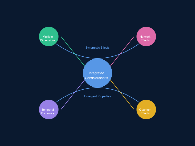
11. Synthesis: The Full Dynamical Picture

The complete framework is a coupled system of:

1. Category theory — structural relationships between assemblies, the biological/technological distinction, functors between consciousness types
2. Game theory — common-payoff structure, immune mechanisms, extended Nash equilibrium with exit strategies
3. Stochastic processes — hypervisor as CTMC, personality as stationary distribution, Monte Carlo exploration of free choices
4. Dynamical systems — coupled circumstance-hypervisor evolution, strange attractors as personality, Lyapunov exponents as unpredictability
5. Differential geometry — Ricci flow on attention manifold, curvature as cognitive habit, singularities as fixation/insight, surgery as therapy
6. Gauge theory — automorphism group as freedom, gauge orbits as equivalent choices, statistical determinism from individual freedom
7. Ideometrics — ideas as granular volume, cogs as capacity for volume, compression as expertise, sacrifice as consolidation

The unifying object is the cognitive assembly (B, μ, T, Σ) with its extended dynamics: the hypervisor evolves stochastically, the attention manifold deforms via Ricci flow, the agent pool changes through sacrifice dynamics, the whole system traces strange attractors in the coupled state space, and all of it is organized by the survival lexicographic order that defines what “rational” means for an embodied, mortal, feeling system.

---

Appendix A: Notation Summary

Symbol	Name	Domain	Definition
B	Agent bag	Finite multiset	The pool of cognitive agents
μ	Marking function	B → {0,1}	Identifies the hypervisor
T	Transfer operator	B × Ω → B	Hypervisor selection rule
Σ	Substrate	Physical medium	Shared realization medium
Iᵢ	Intelligence vector	ℝ⁸₊	Agent i’s capacity in each mode
sᵢ	State filter	[0,1]⁸	Momentary attenuation
λᵢ	Attention allocation	Δ⁷	Distribution over modes
Fᵢ	Experiential fiber	Set	Agent i’s phenomenal states
vᵢ	Vitality function	[0,1]	Agent i’s persistence capacity
cᵢ	Competence function	Ω × O → [0,1]	Agent i’s fitness for role
α	Responsiveness	ℝ₊	Speed of hypervisor swaps
β	Sharpness	ℝ₊	Sensitivity of swap trigger
π	Stationary distribution	Δⁿ⁻¹	Long-run hypervisor frequencies
g_{τσ}	Attention metric	Sym⁺(8)	Riemannian metric on Δ⁷
G(ω)	Gauge group	Subgroup of Aut(B)	Freedom-preserving symmetries
ψᵢ	Self-destructive exit	Strategy	Overwhelm-driven withdrawal
χᵢ	Benevolent sacrifice	Strategy	System-benefiting withdrawal
Ωᵢ	Overwhelm function	ℝ₊	Accumulated unmet demand
θ_ψ	Exit threshold	ℝ₊	Overwhelm tolerance
κ_{ij}	Transfer kernel	[0,1]	Resource redistribution weights
CR	Compression ratio	ℝ₊	Cognitive token efficiency
H	Health metric	ℝ₊	Assembly health score
M	Maturity index	ℝ₊	Geometric smoothness of attention

Appendix B: Open Problems

1. Calibration of the cog unit: No standard instrument exists. Most promising approach: Bayesian updating from task performance batteries.
2. Empirical measurement of the transfer operator T: What neuroscientific observables correspond to hypervisor swaps? Candidate: default mode network transitions.
3. Characterization of the strange attractor for specific personality types: Map clinical personality categories (Big Five, MBTI correlates) to attractor topology.
4. Computation of optimal pruning: The optimal pruning problem is NP-hard in general. Are there biologically plausible approximation algorithms? Does the brain use simulated annealing?
5. Gauge group measurement: Can we experimentally detect the dimension of free will (dim_F) through choice tasks with controlled competence equalization?
6. Sacrifice cascade thresholds: What determines θ_ψ in biological systems? Is it genetically fixed, experience-dependent, or dynamically regulated? Clinical implications for burnout and collapse prevention.
7. The C₁/C₂ boundary: Is there a continuous transition between phenomenal and executive consciousness, or is C₂ a discrete emergence from C₁?
8. Cross-assembly interaction: How do two cognitive assemblies interact? Marriage, teams, and societies as assembly-of-assemblies with their own hypervisor dynamics. Recursive application of the framework to social systems.

---

This working paper is part of the Intelligence as Geometry (IAG) research program.